Earth System Foundation Model (ESFM):
A unified framework for heterogeneous data integration and forecasting

Firat Ozdemir¹, Yun Cheng¹, Salman Mohebi¹, Fanny Lehmann^2,5,
Simon Adamov^3,6, Zhenyi Zhang⁴, Leonardo Trentini⁴, Dana Grund^5,6,
Oliver Fuhrer^3,6, Torsten Hoefler⁷, Siddhartha Mishra⁵,
Sebastian Schemm⁸, Benedikt Soja⁴, Mathieu Salzmann¹

¹Swiss Data Science Center (SDSC), ETH Zurich & EPFL ²ETH AI Center, ETH Zurich ³MeteoSwiss
⁴Institute of Geodesy and Photogrammetry, ETH Zurich ⁵Computational and Applied Mathematics Lab (CAML), ETH Zurich
⁶Institute for Atmospheric and Climate Science (IAC), ETH Zurich ⁷Scalable Parallel Computing Lab (SPCL), ETH Zurich
⁸Dept. of Applied Mathematics and Theoretical Physics, University of Cambridge

arXiv Paper Code Weights

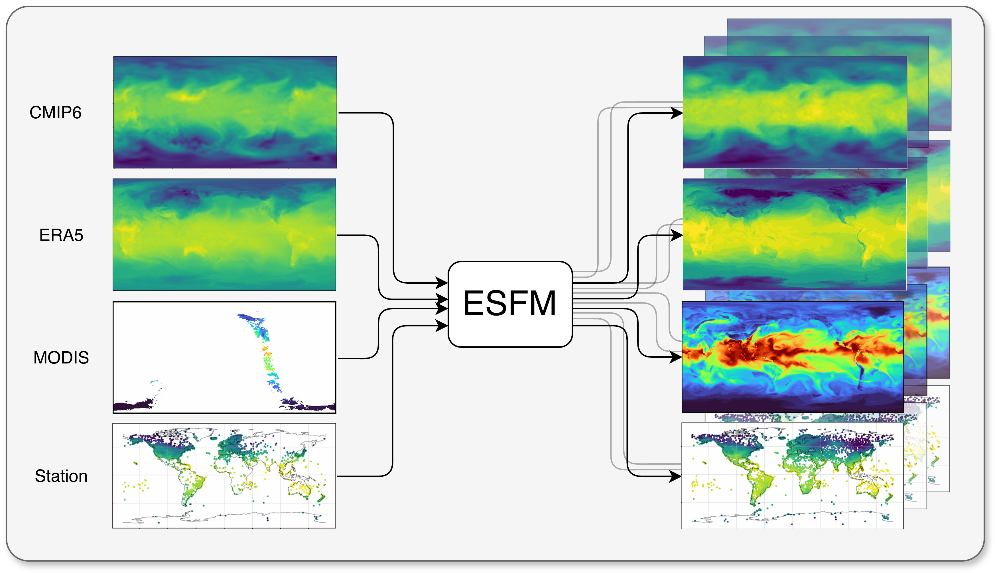
ESFM is a flexible foundation model that ingests multi-modal heterogeneous datasets — dense gridded reanalysis, climate-model output, sparse satellite swaths, and irregular station data — and produces ensemble forecasts, all using the same backbone.

Abstract

Following their success in other areas, such as language processing, the idea of creating a foundation model for natural sciences has gained traction. A foundation model for the Earth system is one that has learned the statistical relationships between physical variables and can predict them. It is a versatile model that excels when finetuned to specific tasks, and not a task-specific weather forecasting model. To achieve this, foundational models are typically pre-trained on very large datasets. Here, we introduce Earth System Foundation Model (ESFM), a fully open model that builds on the 3D Swin UNet transformer backbone of the pioneering Aurora model. ESFM introduces a series of extensions that significantly increase its functionality, thereby fostering the adoption of foundation models in the climate sciences. Firstly, the encoding scheme and training protocols have been extended to handle diverse datasets, including those containing missing values across all spatio-temporal dimensions such as satellite data, as well as station data, all under one backbone. Axial attention is introduced to capture inter-variable dependencies. As a result, ESFM skillfully predicts variables in regions or on pressure levels where no data is present at the initial time, while preserving inter-variable relationships, for example between temperature, pressure, and humidity. Individual variable tokenization enables different sets of variables to be shuffled during training and simplifies the process of building extensions for new downstream tasks. Adaptive layer norm-based ensembles allow for a simple yet effective way to transform deterministic ESFM to a probabilistic FM. We present our findings using dense gridded data, such as ERA5 and CMIP6, as well as regionally masking of dense data, sparse gridded MODIS satellite data, and station data. Our results demonstrate competitive or superior performance relative to state-of-the-art benchmarks in each domain. Additional case studies of Super Typhoon Doksuri in July 2023 and the 2024 sudden stratospheric warming events show clear indications of accurate positional and magnitude estimations of extreme weather. The results show that ESFM retains all the strengths of previous foundation models, such as long term stability, but facilitates the application of foundation models on a variety of downstream tasks.

Key Contributions

Missing data, by design

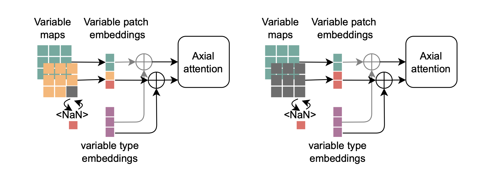
Variable-specific tokenization, together with learnable NaN tokens let ESFM accept observations that are partially or completely missing across any dimension — variable, pressure level, or region.

One backbone, many modalities

Multi-resolution tokenizers group observations into their respective resolution ranges — coarser CMIP6 datasets, 0.25° ERA5 and sparse satellite data, and in-situ station measurements on an irregular grid — all sharing a single 3D Swin UNet processor backbone.

Probabilistic via AdaLN-Zero

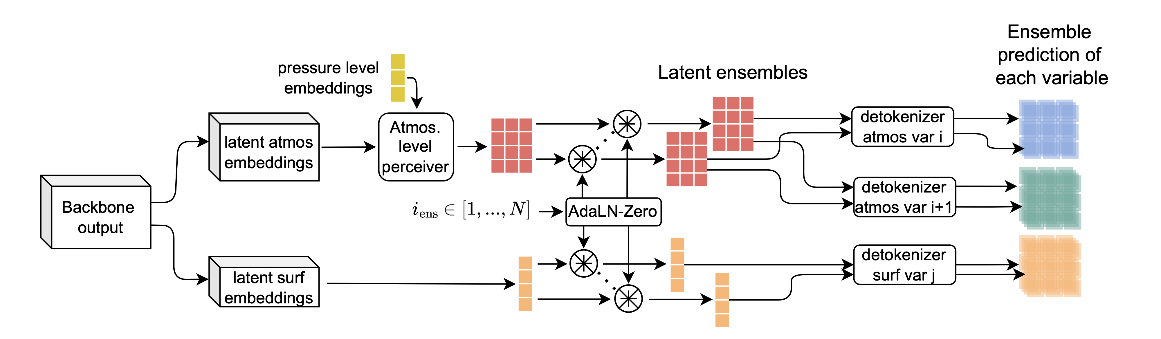
A scale-and-shift modulation on the backbone latents turns deterministic ESFM into an ensemble at negligible cost — extendable to thousands of members without re-running the backbone.

Fully open community model

Training scripts, pretrained weights, and pre-processing code are released — the goal is to lower the barrier for the climate community to finetune ESFM on their own downstream tasks.

Architecture

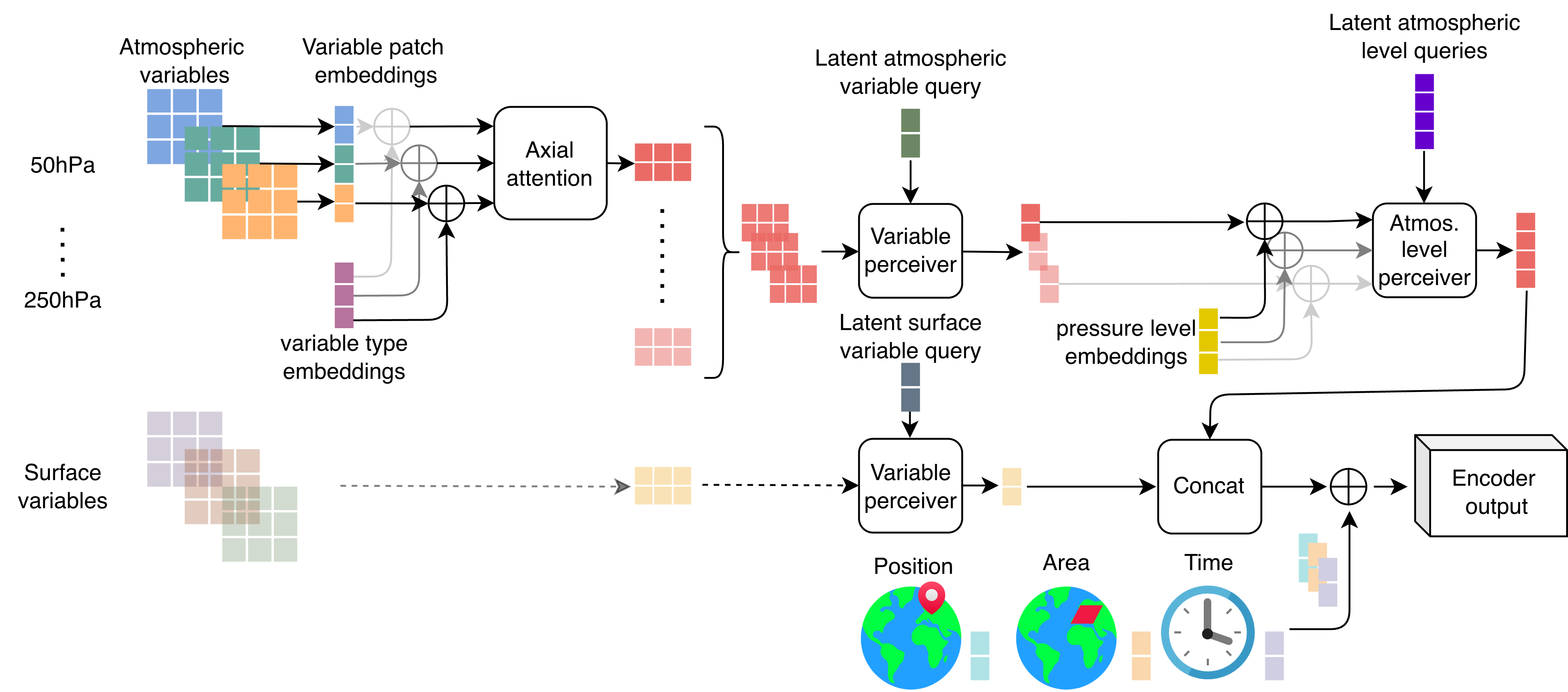
ESFM tokenizes each input variable independently, then runs axial attention across variable tokens before a Perceiver module reduces the latent variable dimension. Atmospheric and surface tokens flow through separate Perceiver paths; atmospheric tokens are further compressed along pressure levels using a separate Perceiver module, inherited from Aurora.

Encoder

Encoder. Variable-specific tokenization → axial attention → Perceiver compression (variable, then pressure-level for atmospheric tokens). Variable-type, position, area, time, and pressure-level embeddings are added throughout.

Handling missing data

Missing-data tokens. Partial (left) or completely missing (right) input patches are replaced with a learnable NaN token (red) that still receives the corresponding variable-type and positional embeddings.

Decoder with AdaLN-Zero ensembles

Decoder. A pressure-level Perceiver maps latent atmospheric embeddings to queried target levels (which do not need to match the input levels). AdaLN-Zero modulates the latents per ensemble member, then shared detokenizers reconstruct variable patches. Zero-initialization makes the deterministic→ensemble extension smooth and non-destructive.

Forecasting Across Heterogeneous Data

The same ESFM backbone can handle dense reanalysis with held-out regions, sparse satellite swaths, and irregular station data — without architectural changes.

Masked ERA5 — Forecasting Continents With No Initial Data

All variables across Europe are removed from the initial conditions. ESFM still produces a physically consistent forecast inside the masked region, with geostrophic balance and T–Q saturation envelopes preserved (see Sec. 5.1 of the paper).

MODIS Sparse Satellite — Dense Global PWV from a Narrow Swath

At any given hour, MODIS observes only ~3% of the globe (a narrow polar-orbit swath). ESFM finetuned on MODIS produces a globally dense precipitable-water-vapor forecast and remains stable in 2-week autoregressive rollouts initialized from the sparse observations.

Weather Stations — Irregular, In-Situ Forecasting

Station data is greedily mapped to an irregular 90×180 grid (with exact positional encoding preserved) and tokenized at 1×1 patches. ESFM matches SotA station benchmark leader models on Weather-5K and generalizes to held-out stations unseen during training on ECMWF11k dataset.

Case Study I — Super Typhoon Doksuri (July 2023)

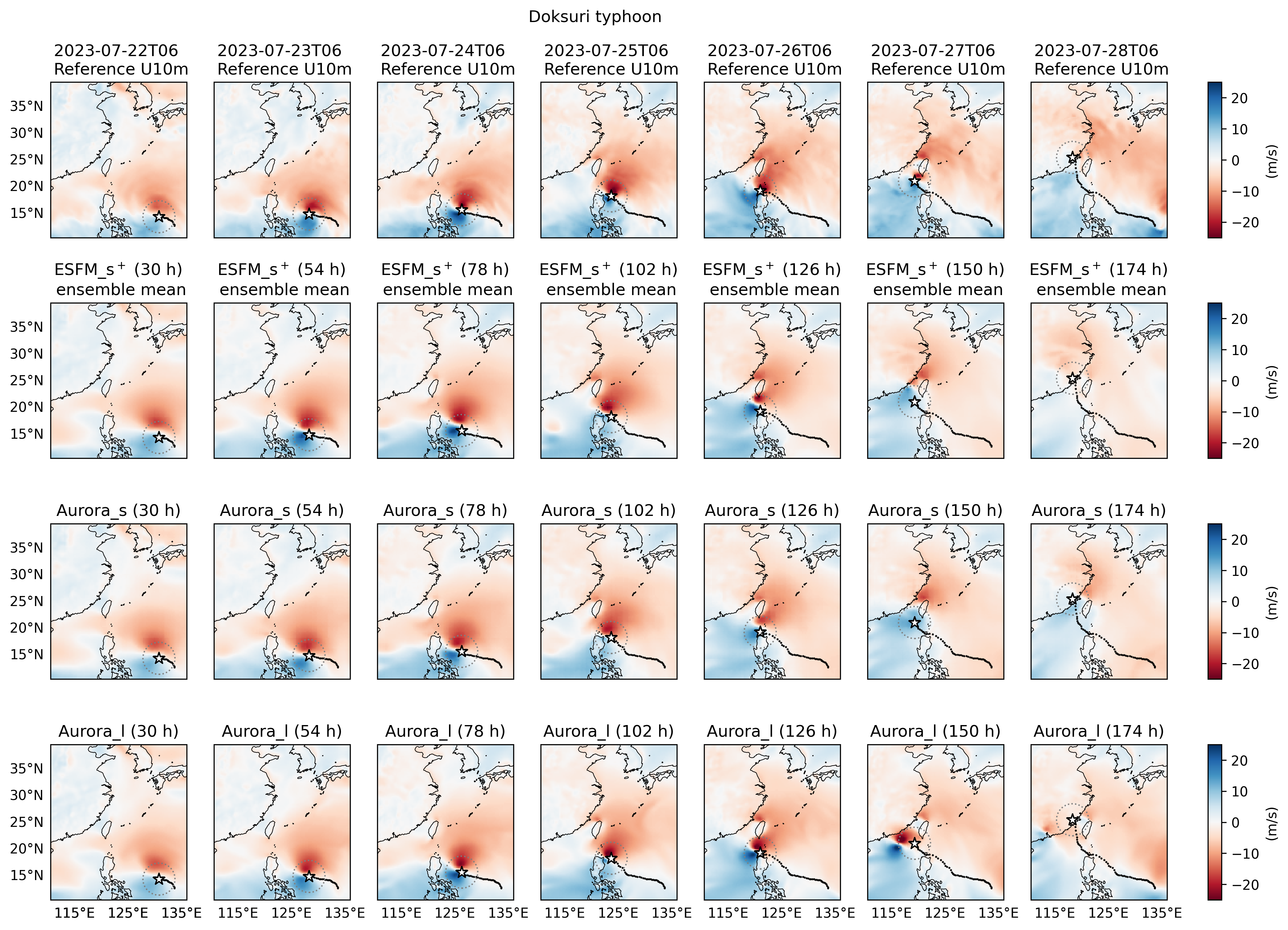
Doksuri is an exceptionally powerful out-of-training-set typhoon. MLWP models typically forecast cyclone position well but underestimate intensity. Despite having the parameter count of Aurora_s, the probabilistic ESFM_s⁺ ensemble tracks the IBTrACS reference track closely for up to 174 h rollout, demonstrating strong localization and intensity performance compared to Aurora_s and Aurora_l.

Doksuri U10m track — ERA5 reference and ensemble means

10-meter eastward wind (U10m) during Super Typhoon Doksuri — ERA5 reference track alongside ensemble means from ESFM_s⁺, Aurora_s, and Aurora_l for up to 174 h rollout. ESFM_s⁺ achieves strong localization and intensity tracking despite matching the model size of Aurora_s.

Case Study II — Sudden Stratospheric Warmings 2023/24

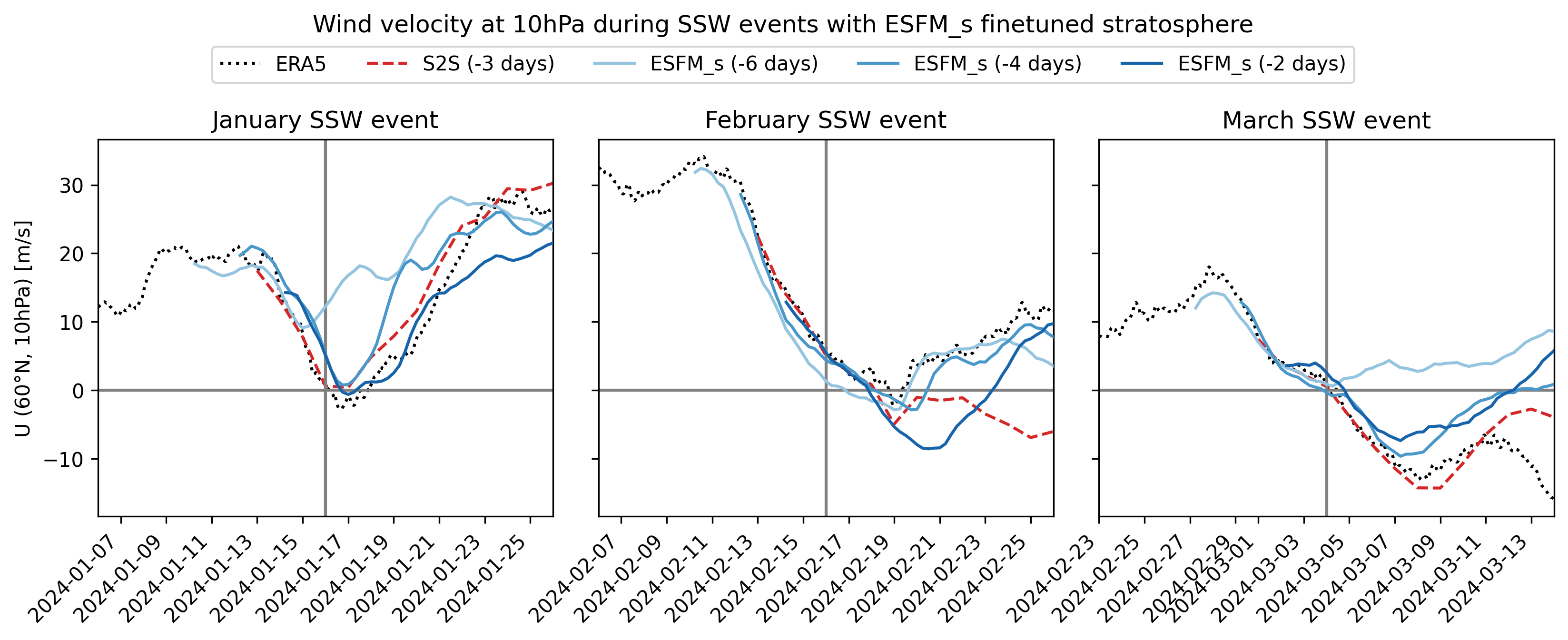
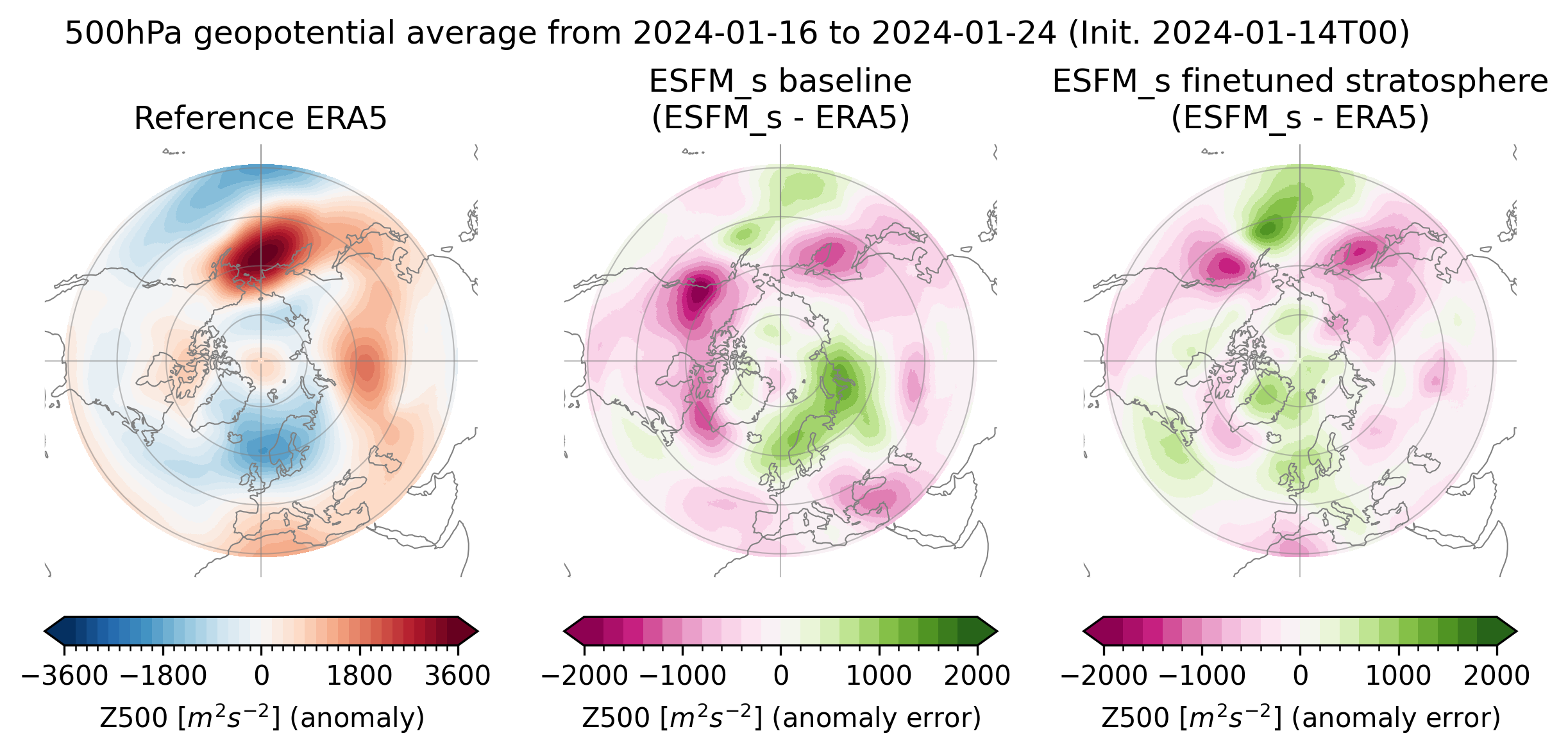
The stratosphere strongly modulates surface weather on sub-seasonal timescales, but most data-driven models stop at 50 hPa. We finetuned ESFM with 16 pressure levels (adding 10, 20, and 70 hPa). This lead to more skillful prediction of the zonal-wind reversal during three SSW events, comparable to ECMWF's numerical S2S model — and an improved tropospheric response (500 hPa geopotential anomaly) over the baseline.

Eastward wind at 10 hPa, 60°N during the Jan/Feb/Mar 2024 SSW events.

500 hPa geopotential anomaly the week after the January SSW — the stratosphere-finetuned ESFM (right) recovers the ridge/trough pattern more accurately than baseline.

Multi-Decadal Stability

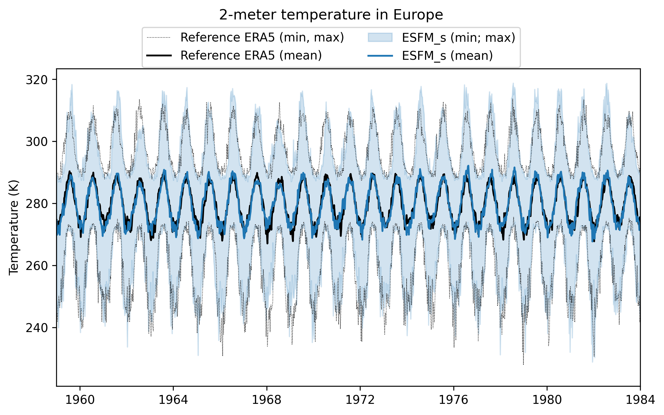
A 25-year autoregressive rollout initialized on 02.01.1959 remains stable, preserves the seasonal cycle, and tracks the ERA5 climatology of European 2-meter temperature — without manual constraints on mass or energy balance. This long-term stability is inherited from Aurora's backbone and preserved through ESFM's architectural changes.

25-year rollout of 2m temperature over Europe

25-year rollout of 2-meter temperature over Europe. Solid line: spatial mean; shaded: spatial min–max. ERA5 reference in gray/black. Points sampled every 7 days.

Implicit Physics

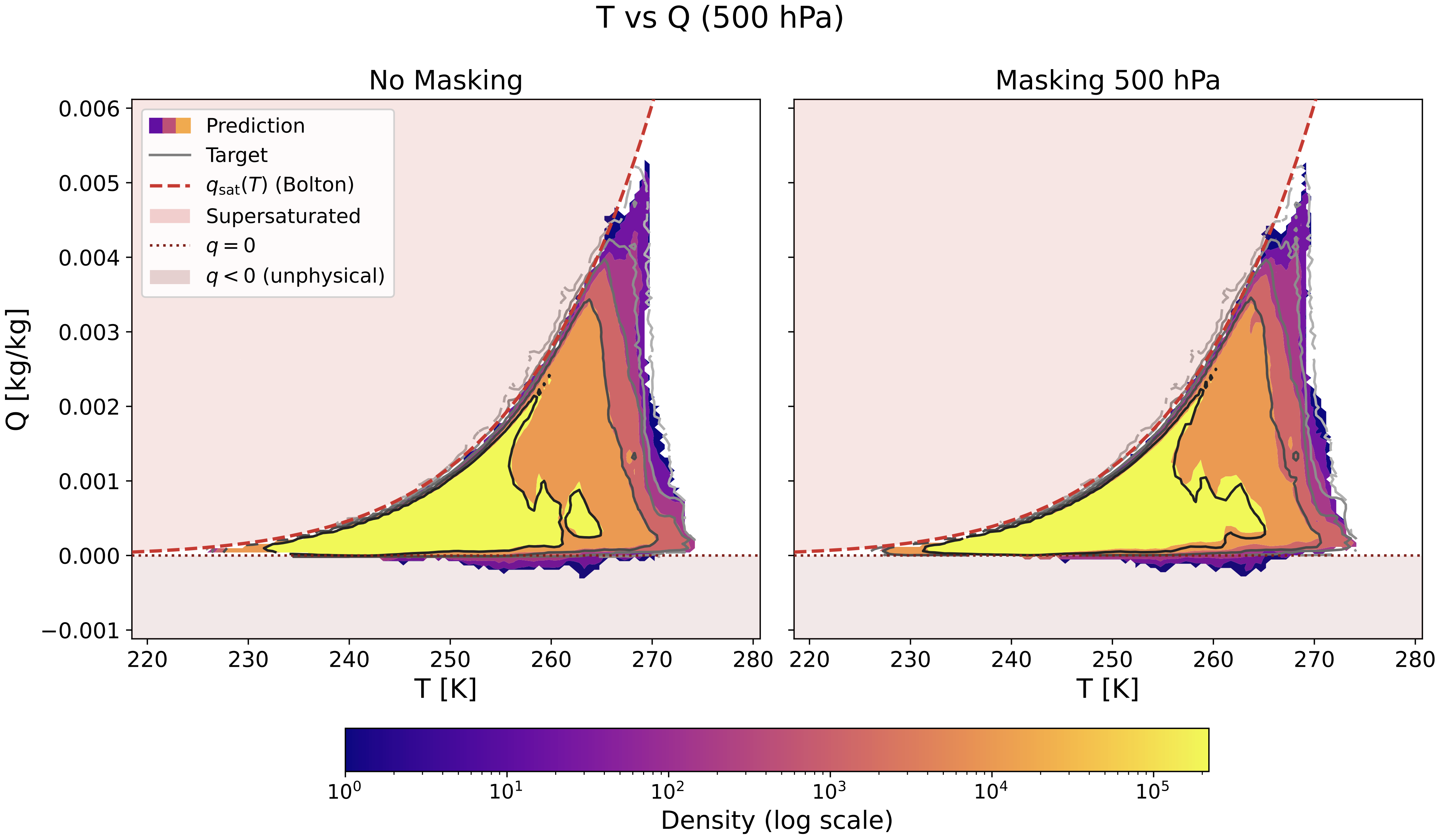
Neither the Clausius–Clapeyron envelope nor geostrophic wind balance is enforced during training. Yet when an entire pressure level or a whole continent is held out from the initial conditions, ESFM's joint distributions of T–Q and |∇GH|–wind speed remain physically plausible, tracking the saturation curve and geostrophic slope respectively.

Joint density of T and Q at 500 hPa over Europe, with no masking (left) vs. the full 500 hPa level held out from initial conditions (right). Predictions stay below Bolton's q_sat(T).

ERA5 Benchmarks

ESFM_s (~110M params, matching Aurora_s) is on par with AIFS and Aurora_s on dense ERA5 forecasting, outperforms GraphCast, SFNO, and IFS control for surface variables, while retaining the flexibility to handle missing/sparse/station data with the same backbone. Below is a 6-hour MAE comparison; see the paper for full rollout and CRPS metrics.

Model	T850	Z500	Q850	T2m	U10m	V10m
ESFM_s	0.224	12.535	2.24e-4	0.248	0.253	0.262
Aurora_s	0.218	13.825	2.18e-4	0.246	0.256	0.262
Aurora_l	0.167	11.687	1.76e-4	0.194	0.195	0.201
AIFS	0.182	14.679	1.90e-4	0.219	0.232	0.238
GraphCast	0.208	13.608	2.08e-4	0.304	0.269	0.272
SFNO	0.217	13.852	2.17e-4	0.255	0.282	0.294
IFS Control	0.346	15.804	3.90e-4	0.421	0.433	0.444

6-hour lead-time MAE on the ERA5 test set. Lower is better.

Station Data Benchmarks

ECMWF 11k Station Data

We evaluate ESFM_s on the 11,863 ECMWF station dataset (trained on samples between 2000 and 2020). The dataset is unimputed and sparse: temperature occupancy ranges from ~0% to 99.3% across stations (median 66.1%), while sea-level pressure has a median occupancy of only 29.1%. We hold out 1 k stations completely during training and test under three regimes: regular evaluation (trained station locations in the test period), holdout station I/O (novel stations introduced at test time), and extrapolating holdout stations (novel locations inferred from trained station observations only, with no observations provided at the new coordinates).

Evaluation	Lead time	T		dT		U		V		MSL		WS		WD
Evaluation	Lead time	MAE	PCC	MAE	PCC	MAE	PCC	MAE	PCC	MAE	PCC	MAE	PCC	MAE	PCC
Regular evaluation	6h	1.07	0.98	1.18	0.98	1.18	0.86	1.18	0.85	76.89	0.98	1.04	0.83	34.26	0.68
	12h	1.24	0.98	1.38	0.97	1.32	0.82	1.32	0.82	126.63	0.97	1.13	0.80	36.68	0.65
	24h	1.56	0.97	1.75	0.96	1.63	0.72	1.63	0.71	248.58	0.90	1.34	0.72	44.58	0.58
Holdout station I/O	6h	1.87	0.97	1.63	0.97	1.77	0.75	1.76	0.72	148.75	0.96	1.57	0.68	47.85	0.54
	12h	2.05	0.97	1.93	0.96	1.98	0.68	1.95	0.64	196.65	0.94	1.74	0.60	51.92	0.51
	24h	2.20	0.96	2.21	0.95	2.18	0.59	2.16	0.53	308.78	0.85	1.83	0.53	57.48	0.46
Extrapolating holdout stations	6h	2.32	0.94	2.37	0.92	2.02	0.64	1.97	0.61	177.09	0.92	1.81	0.55	53.69	0.43
	12h	2.36	0.94	2.44	0.93	2.09	0.62	2.03	0.60	211.29	0.90	1.87	0.54	55.06	0.41
	24h	2.50	0.94	2.64	0.92	2.28	0.54	2.20	0.52	302.12	0.85	1.96	0.48	60.12	0.36

Forecast MAE (lower is better) and PCC (higher is better) for ESFM_s on ECMWF 11k station variables: temperature (T), dew point (dT), eastward/northward wind (U/V), sea-level pressure (MSL), wind speed (WS), wind direction (WD).

Weather-5K Station Data

Weather-5K is an imputed benchmark with ~5 k globally distributed stations (training set covering 2014–2021). Baseline models receive 48 h of temporal history and predict target lead times directly without autoregressive rollouts. Despite using its default (t−Δt, t) two-frame observation setup, ESFM_s remains competitive, especially at short lead times.

Model	Lead time	Temperature	Dewpoint	Wind speed	Wind direction	Sea level pressure	Overall
ESFM_s	6h	1.10	1.17	1.06	36.44	0.62	8.1
ESFM_s	12h	1.32	1.45	1.16	39.32	1.23	8.9
ESFM_s	24h	1.76	1.86	1.40	46.29	2.55	10.8
Pyraformer	24h	1.75	1.83	1.30	61.8	1.90	13.7
iTransformer	24h	1.82	1.93	1.32	63.2	1.99	14.1
Informer	24h	1.88	1.94	1.30	60.7	2.01	13.6
Autoformer	24h	1.93	2.06	1.42	66.5	2.26	14.8
FEDformer	24h	1.98	2.02	1.36	66.0	2.13	14.5

MAE on Weather-5K (lower is better). Wind speed and direction for ESFM_s are derived from U and V components. Overall score is the average of the five variables.

Quickstart

ESFM runs inside a container environment (tested on physicsnemo:25.03 on CSCS Alps). To get started, clone the repository and build the Dockerfile to obtain a compatible runtime.

git clone https://github.com/swiss-ai/ESFM

Interactive inference: for a quick ERA5 visualisation using model weights from Hugging Face and a desired init condition from WeatherBench2, have a look at the notebook (we are working on providing a conda environment configuration for simple local inference):

notebooks/inference_ESFMs_on_ERA5.ipynb

Script-based inference: set your data path prefix, then run the inference entrypoint with an experiment config:

export ESFM_DATA_PATH_PREFIX=/your/storage/root
python inference_rollout.py \
    --config ./configs/config_ESFM_s_nm.yaml \
    --NUM_ROLLOUT_STEPS 56

See the repository README for training recipes, Slurm scripts, masking configurations, and instructions for plugging in your own dataset (gridded, sparse, or station-based).

Reproducing Experiments

Detailed instructions for reproducing the ESFM training and inference experiments from the paper — including checkpoint notes, Slurm script usage, and environment setup — are available in scripts/README.md.

BibTeX

@article{ozdemir2026esfm,
  title   = {ESFM: A Unified Earth System Foundation Model for Heterogeneous Data Integration and Forecasting},
  author  = {Ozdemir, Firat and Cheng, Yun and Mohebi, Salman and Lehmann, Fanny and
             Adamov, Simon and Zhang, Zhenyi and Trentini, Leonardo and Grund, Dana and
             Fuhrer, Oliver and Hoefler, Torsten and Mishra, Siddhartha and Schemm, Sebastian and
             Soja, Benedikt and Salzmann, Mathieu},
  journal = {arXiv preprint arXiv:submit/7499478},
  year    = {2026}
}

Acknowledgments

This work was supported under project IDs a01 and a122 as part of the Swiss AI Initiative, through a grant from the ETH Domain and computational resources provided by the Swiss National Supercomputing Centre (CSCS) under the Alps infrastructure. Contributions of F. Lehmann were primarily supported by the ETH AI Center through their ETH AI Center postdoctoral fellowship. Contributions of L. Trentini were supported by the Swiss National Science Foundation (SNSF) under grant number 225851. The authors thank sincerely A. Zoller for running ensemble rollout forecasts of the compared SotA models and L. Huang for insightful discussions throughout the development of ESFM.

Earth System Foundation Model (ESFM): A unified framework for heterogeneous data integration and forecasting